Jupyter Notebooks
One of the most widespread, powerful and useful tools used through the fields of Data Science and Machine Learning is Jupyter Notebooks.
In this post I am going to briefly explain what they are and some ways in which you can start working with them.
What is a Jupyter Notebook?
An open-source web-based interactive computational environment
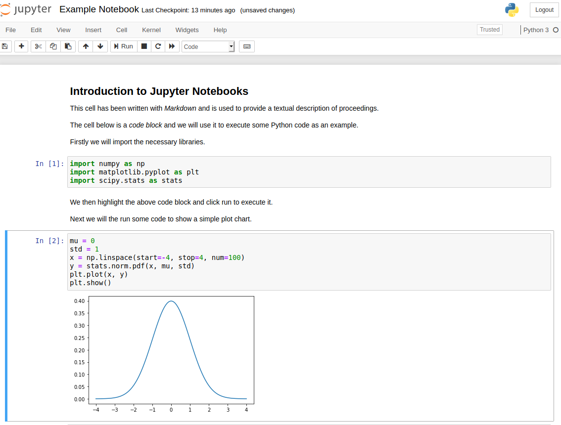
that enables users to create and share documents that contain live code,
equations, visualisations, images, video, interactive widgets and narrative text.
The Jupyter Notebook comprises of three components:
The notebook web application: An interactive web application for writing and running code interactively and authoring notebook documents.
Kernels: Separate processes started by the notebook web application that runs users’ code in a given language and returns output back to the notebook web application. The kernel also handles things like computations for interactive widgets, tab completion and introspection.
Notebook documents: Self-contained documents that contain a representation of all content visible in the notebook web application, including inputs and outputs of the computations, narrative text, equations, images, and rich media representations of objects. Each notebook document has its own kernel.
Notebook web application
The notebook web application enables users to:
- Edit code in the browser, with automatic syntax highlighting, indentation, and tab completion/introspection.
Run code from the browser, with the results of computations attached to the code which generated them.
See the results of computations with rich media representations, such as HTML, LaTeX, PNG, SVG, PDF, etc.
Create and use interactive JavaScript widgets, which bind interactive user interface controls and visualizations to reactive kernel side computations.
Author narrative text using the Markdown markup language.
Include mathematical equations using LaTeX syntax in Markdown
Kernels
Jupyter Notebooks are language agnostic and support execution environments (aka kernels) across many different programming languages which include Python, Julia, R.
For each notebook document that a user opens, the web application starts a kernel that runs the code for that notebook. Each kernel is capable of running code in a single programming language only.
For our purposes, we will be focusing on the Python programming language, which is the default.
Notebook documents
A Jupyter Notebook document is a JSON document, following a versioned schema, and containing an ordered list of input/output cells which can contain code, text (using Markdown), mathematics, plots and rich media, usually ending with the “.ipynb” extension.
A Jupyter Notebook can be converted to a number of open standard output formats (HTML, presentation slides, LaTeX, PDF, ReStructuredText, Markdown, Python)
Notebook documents contain the inputs and outputs of an interactive session as well as narrative text that accompanies the code but is not meant for execution. Rich output generated by running code, including HTML, images, video, and plots, is embedded in the notebook, which makes it a complete and self-contained record of a computation.
When you run the notebook web application on your computer, notebook documents are just files on your local filesystem with a .ipynb extension. This allows you to use familiar workflows for organizing your notebooks into folders and sharing them with others.
Notebooks consist of primary types of cells:
Code cells: Input and output of live code that is run in the kernel
Markdown cells: Narrative text containing Plain text, HTML, Markdown, images, videos or LaTeX.
Where can I find Jupyter Notebooks?
There are numerous ways in which you can run your own Jupyter Notebooks, of which just a few are mentioned below:
- Install your own Jupyter Notebook server
- Run a Docker container that is already preconfigured with a Jupyter Notebook server
- On AWS using Amazon Sagemaker Notebooks
- On Azure using Azure Notebooks
- On Google Cloud using Colaboratory
Having your own installation is the most customisable option for the power user but it is often also one of the most complex. One way to alleviate some of that installation pain whilst also being able to harness the flexibility offered by this method of operation is to make use of Docker containers and I will go into this in a bit more detail in a bit.
Public Cloud providers also offer options for use of Notebook services.
AWS offer the Sagemaker managed service which include Notebooks and gives the options of dozens of pre-built notebooks for different use cases. There are also hundreds of algorithms and pre-trained models available within the AWS Marketplace to make it easy to get started quickly.
AWS offer two months of free (maximum of 250hrs per month) usage of Sagemaker Notebooks as part of their Free Tier but there is a cost applicable after that.Azure Notebooks is a free service that offers environments with Python, R and F kernels. However each project is each project is limited to 4GB memory, 1GB data and is only guaranteed to last for up to an 8 hr session before it might time out.
Google offer a service called Colaboratory which is a fork of the Jupyter application although it works in the same way. It has some limitations such as being focused on support for the Python kernel however it free access to higher specification computing resources than Azure which includes GPUs as well as guaranteeing it wont time out for up to 12 hrs.
I hope this guide has been informative for you, in my next post we will get started in playing around with our own Jupyter Notebook.
